| |
Knowledge Center |
| |
The most important thing when dealing with investment returns is to bear in mind that what is measured are past returns and that it is very unlikely that the past will be ever repeated in the future.
From a calculation point of view, it is important to keep in mind that investment returns are nothing more than growth rates of the capital invested over a certain time period expressed as a percent figure.
The rate of return can be calculated over a single period, or expressed as an average over multiple periods of time. |
| |
The arithmetic return is:
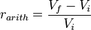
rarith is sometimes referred to as the yield. |
| |
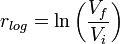
The logarithmic return or continuously compounded return is defined as:
 |
| |
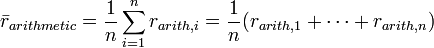
The arithmetic average rate of return over n periods is defined as:
 |
| |
The geometric average rate of return, also known as the True Time-Weighted Rate of Return, over n periods is defined as:
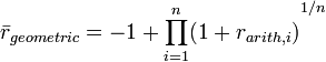
The geometric average rate of return calculated over n years is also known as the annualized return.
Some relationship: GM ~ AM – (Variance/2) |
| |
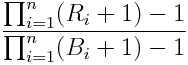
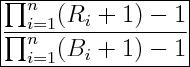
The CAGR is defined as the year-over-year growth rate of an investment over a specified period of time.
The compound annual growth rate is calculated by taking the nth root of the total percentage growth rate, where n is the number of years in the period being considered. This can be written as follows:
Investors can compare the CAGR in order to evaluate how well one investment performed against other investment in a peer group or against a market index. The CAGR can also be used to compare the historical returns of stocks to bonds or a portfolio. But the CAGR does not reflect investment risk, it smooth out the return thus hiding the volatility. |
| |
Standard deviation is a widely used measurement of variability or diversity used in statistics and probability theory. It shows how much variation or "dispersion" there is from the average (mean, or expected value). A low standard deviation indicates that the data points tend to be very close to the mean, whereas high standard deviation indicates that the data are spread out over a large range of values.
The most common estimator for σ used is an adjusted version, the sample standard deviation, denoted by s and defined as follows:
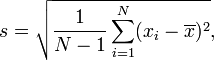
Where  are the observed values of the sample items and are the observed values of the sample items and  is the mean value of these observations. is the mean value of these observations.
The significance of standard deviation is that two-third of the times the annual return of the asset lies between +1 SD and -1 SD from mean, 95% of time lies between +2 SD and -2SD and 99% of time lies between +3 SD and -3 SD in a normal distribution. |
| |
The standard error is a method of measurement or estimation of the standard deviation of the sampling distribution associated with the estimation method. The term may also be used to refer to an estimate of that standard deviation, derived from a particular sample used to compute the estimate.
The standard error of the mean (i.e., of using the sample mean as a method of estimating the population mean) is the standard deviation of those sample means over all possible samples (of a given size) drawn from the population. Secondly, the standard error of the mean can refer to an estimate of that standard deviation, computed from the sample of data being analyzed at the time.

Where, σ is the standard deviation of the population.
The smaller the standard error, the more representative the sample will be of the overall population. The standard error is also inversely proportional to the sample size; the larger the sample size, the smaller the standard error because the statistic will approach the actual value. |
| |
The coefficient of variation represents the ratio of the standard deviation to the mean, and it is a useful statistic for comparing the degree of variation from one data series to another, even if the means are drastically different from each other. It is also known as unitized risk or the variation coefficient. The absolute value of the CV is sometimes known as relative standard deviation (RSD), which is expressed as a percentage.
The coefficient of variation (CV) is defined as the ratio of the standard deviation  to the mean to the mean  : :

It shows the extent of variability in relation to mean of the population.
In the investing world, the coefficient of variation allows you to determine how much volatility (risk) you are assuming in comparison to the amount of return you can expect from your investment. In simple language, the lower the ratio of standard deviation to mean return, the better your risk-return tradeoff. |
| |
In probability theory and statistics, skewness ('3rd moment of a distribution') is a measure of the asymmetry of the probability distribution of a real-valued random variable. The skewness value can be positive or negative, or even undefined.
A symmetric distribution has zero skewness, an asymmetric distribution with the largest tail to the right has positive skewness, and a distribution with a longer left tail has negative skewness.
Positive skewness = Mode < Median < Arithmethic Mean, Negative Skewness = Mode > Median > Arithmethic Mean, Symmetrical = Arithmetic Mean = Median
Moment coefficient of skewness of a data set is
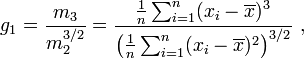
Where,
m3 = ∑(x−x̄)3 / n and m2 = ∑(x−x̄)2 / n
x̄ is the mean and n is the sample size, as usual. m3 is called the third moment of the data set. m2 is the variance, the square of the standard deviation.
If skewness is positive, the returns are positively skewed or skewed right, meaning that the right tail of the distribution is longer than the left. If skewness is negative, the returns are negatively skewed or skewed left, meaning that the left tail is longer. |
| |
The classical interpretation of Kurtosis is that it measures both peakedness and tail heaviness of a distribution relative to that of the normal distribution. Consequently, its use is restricted to symmetric distributions.
The moment coefficient of kurtosis of a data set is computed almost the same way as the coefficient of skewness: just change the exponent 3 to 4 in the formulas:
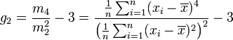
Where
m4 = ∑(x−x̄)4 / n and m2 = ∑(x−x̄)2 / n
Excess kurtosis: g2 = a4−3
m4 is called the fourth moment of the data set. m2 is the variance, the square of the standard deviation. xi is the ith value, and  is the sample mean. is the sample mean.
Again, the excess kurtosis is generally used because the excess kurtosis of a normal distribution is 0.
Normal-distributed returns have a kurtosis of 0, irrespective their mean or standard deviation. Distributions with kurtosis of 3 are said to be mesokurtic. If a distribution’s kurtosis is greater than 3, it is said to be leptokurtic. If its kurtosis is less than 3, it is said to be platykurtic. Leptokurtosis is often associated with distributions that are simultaneously “peaked” and have “short tails.” Platykurtosis is often associated with distributions that are simultaneously "less peaked" and have "long tails".
The smallest possible kurtosis is 1 (excess kurtosis −2), and the largest is ∞. For a return distribution a negative excess kurtosis (platykurtic) is prefers over positive excess return (leptokurtic). |
| |
In probability theory and statistics, covariance is a measure of how much two variables change together. Variance is a special case of the covariance when the two variables are identical.
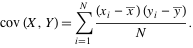
A positive covariance means that asset returns move together. A negative covariance means returns move inversely. Possessing financial assets that provide returns and have a high covariance with each other will not provide very much diversification. |
| |
Correlation is the degree to which two or more quantities are linearly associated. For two random variables X and Y, the correlation is defined by
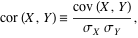
where  denotes standard deviation and denotes standard deviation and  is the covariance of these two variables. is the covariance of these two variables.
Correlation is computed into what is known as the correlation coefficient, which ranges between -1 and +1. Perfect positive correlation (a correlation co-efficient of +1) implies that as one security moves, either up or down, the other security will move in lockstep, in the same direction. Alternatively, perfect negative correlation means that if one security moves in either direction the security that is perfectly negatively correlated will move in the opposite direction. If the correlation is 0, the movements of the securities are said to have no correlation; they are completely random. |
| |
It is a statistic used in the context of statistical models whose main purpose is either the prediction of future outcomes or the testing of hypotheses, on the basis of other related information. It provides a measure of how well observed outcomes are replicated by the model, as the proportion of total variation of outcomes explained by the model
This measure represents the percentage of a fund or security's movements that can be explained by movements in a benchmark index. For fixed-income securities, the benchmark is the NSE T-bill Index. For equities, the benchmark is the CNX Nifty. |
| |
The Sharpe ratio or Sharpe index or Sharpe measure or reward-to-variability ratio is a measure of the excess return (or risk premium) per unit of risk in an investment asset or a trading strategy, named after William Forsyth Sharpe. It is defined as
where R is the asset return, Rf is the return on a benchmark asset, such as the risk free rate of return, E[R − Rf] is the expected value of the excess of the asset return over the benchmark return, andσ is the standard deviation of the excess of the asset return.
The Sharpe ratio is used to characterize how well the return of an asset compensates the investor for the risk taken, the higher the Sharpe ratios number the better. |
| |
Like the Sharpe Ratio, the Treynor Ratio (sometimes called Reward-to-Variability-Ratio) is a measurement of the returns earned in excess of that which could have been earned on an investment that has no diversifiable risk (e.g., Treasury Bills or a completely diversified portfolio), per each unit of market risk assumed.
The Treynor ratio relates excess return over the risk-free rate to the additional risk taken; however, systematic risk is used instead of total risk. The higher the Treynor ratio, the better the performance of the portfolio under analysis.
R = Portfolio return,
Rf = risk free rate
 = Portfolio Beta = Portfolio Beta |
| |
Modigliani Risk-Adjusted Performance or M2 or M2 or Modigliani-Modigliani measure or RAP is a risk-adjusted performance measure. It contains the same information as the Sharpe Ratio, but, being a percentage return, is easier to interpret. It measures the returns of the portfolio, adjusted for the risk of the portfolio, relative to that of some benchmark (e.g., the market).
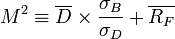
Dt be the excess return of the portfolio (i.e., above the risk-free rate) for some time period t:
It also defined a statistic called "RAPA" (presumedly, Risk Adjusted Performance Alpha). Consistent with the more common terminology of M2, this would be:
Where, S = sharpe ratio. |
| |
The beta coefficient is a key parameter in the capital asset pricing model (CAPM). Beta is that element of return variability from a portfolio which cannot be eliminated through diversification relative to one or several risk factors. It comprises the risk factors common to all assets in the investment universe. That’s why it is also the measure of systematic Risk.
Beta expresses the 'sensitivity' of the portfolio relative to the 'market'. By definition, the "market" has a beta of 1.0. A portfolio that swings more than the market over time has a beta above 1.0. If a portfolio moves less than the market, the portfolios' beta is less than 1.0. High-beta portfolios are supposed to be riskier but provide a potential for higher returns; low-beta portfolios pose less risk but also lower returns.
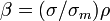
Where β is Beta, σ is the volatility of the security or portfolio, ρ is the correlation of returns of portfolio and the market and σm is market volatility. |
| |
Jensen's alpha (or Jensen's Performance Index, ex-post alpha) is used to determine the return of a security or portfolio of securities over and above the theoretical expected return. The security could be any asset, such as stocks, bonds, or derivatives. The theoretical return is predicted by a market model, most commonly the Capital Asset Pricing Model (CAPM) model. The market model uses statistical methods to predict the appropriate risk-adjusted return of an asset. The CAPM for instance uses beta as a multiplier.
In the context of CAPM, calculating alpha requires the following inputs:
Jensen's alpha = Portfolio Return − [Risk Free Rate + Portfolio Beta * (Market Return − Risk Free Rate)]
 |
| |
Tracking error is a measure of how closely a portfolio follows the index to which it is benchmarked. The most common measure is the root-mean-square of the difference between the portfolio and index returns

Where Rp - Rb is the difference between the portfolio return and the index return.
Tracking Error of a portfolio constantly underperforming its benchmark is zero, for example, and therefore hardly a desirable result. |
| |
The Information Ratio (also known as Appraisal Ratio) is basically a risk-adjustment of Alpha. It measures the Alpha per unit of active risk, i.e. tracking error. It is defined as expected active return divided by tracking error, where active return is the difference between the return of the security and the return of a selected benchmark index, and tracking error is the standard deviation of the active return.
Where,
Rp is the portfolio return, Rb is the benchmark return
α = Active Return
ω (Tracking Error) = sd is the standard deviation of the active return |
| |
A measure of the dispersion of all observations that fall below the mean or target value of a data set. Semivariance is an average of the squared deviations of values that are less than the mean or target value.

Where:
n = the total number of observations below the mean
rt = the observed value
average = the mean value of the data set
Similarly, Semi volatility is defined as the volatility of returns below the mean return. |
| |
Downside volatility takes into account only those values of observed excess rates of return that lie below minimal acceptable return (MAR). In other words, Downside volatility is a generalization of the semi volatility as is defined as volatility below MAR.
 |
| |
This measure of downside risk is colloquially known as "downside risk." The main idea of the lower partial moment framework is to model moments of asset returns that fall below a minimum acceptable level of return.
LPM simply examines the moment of degree ‘a’ below a certain threshold ‘t’.
Where a = order of the lower partial moment
T = target return (Minimum accepted return)
LPM is a family of risk measures specified by‘t’ and ‘a’. ‘T’ is often set to the risk free rate or simply to zero. By choosing the degree of the moment an investor can specify the measure to suit his risk aversion. Intuitively, large values of ‘a’ will penalize large deviations more than low values. Semi variance is a special case of LPM for which the degree of the moment is set to two. |
| |
Up-capture compares an investment’s performance against its benchmark during periods when the benchmark’s performance is positive, while down-capture compares the investment’s performance against the benchmark during periods when the benchmark’s performance is negative.
A value of 100% for either ratio implies that the investment fully captures, or matches, the benchmark return during the period evaluated. A value of greater than 100% indicates that the investment captured more return than the benchmark (this is a positive for up-capture, however, a negative for down-capture). A value less than 100% means the investment captured less return than its benchmark (this is a negative for up-capture, however, a positive for down-capture).
Up- and down-capture ratios are commonly used to determine how much an investment participates in the upside or downside of the market. Theoretically this can help determine if a given investment is more aggressive or defensive in nature, which would help determine the type of investor for which that investment is appropriate. Another common use of these ratios is for investors who make tactical allocations to an investment based on their expectation of future market performance.
The Up Capture Ratio is:
 are the fund returns when the benchmark returns are greater than or equal to zero are the fund returns when the benchmark returns are greater than or equal to zero
 are the benchmark returns when the benchmark returns are greater than or equal to zero are the benchmark returns when the benchmark returns are greater than or equal to zero
The Down Capture Ratio is:
 are the fund returns when the benchmark returns are less than zero are the fund returns when the benchmark returns are less than zero
 are the benchmark returns when the benchmark returns are less than zero are the benchmark returns when the benchmark returns are less than zero
|
| |
It calculates the probability that the portfolio would not achieved the target return (MAR).
Downside Probability = Total number of negative returns in a period/ Total number of returns in a period.
While higher figure is considered bad, lower figure is considered favourable. |
| |
The chance that a manager’s return will equal or exceed the target return (MAR).
Upside Probability = Total number of par or positive returns in a period/ Total number of returns in a period.
|
| |
The average return above the TR, measuring how often and how far above the TR a portfolio’s returns are likely to occur. Upside Potential, a term coined by Nobel Prize winner Daniel Kahneman, captures investors’ perception of risks concerning gains as opposed to risk concerning losses.
 |
| |
The ratio of Upside Potential to Downside Deviation at a given TR, measuring how much upside potential is provided by a manager at a given level of downside risk.
Mathematically,
U-P Ratio = UP / DD
Where,
UP = Upside Potential
DD = downside deviation |
| |


